Q6Advanced Engineering Mathematics
Question
Obtain the optimal transportation plan from the following table:
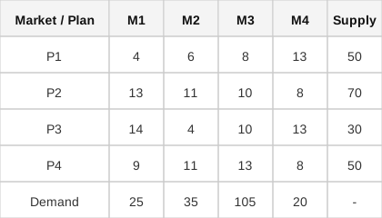
Answer
The transportation problem is resolved by balancing the supply and demand matrices, applying Vogel's Approximation Method for an initial solution, and rigorously optimizing it via the MODI method.
To solve a transportation problem for minimizing total logistical cost, we follow a two-phase algorithmic approach. The first phase establishes a feasible starting point, and the second phase refines it to absolute optimality.
Phase 1: Balancing and Initial Feasible Solution
First, we must meticulously check if the problem is perfectly balanced.
- Total Capacity (Supply): units.
- Total Requirement (Demand): units.
Because Total Supply strictly exceeds Total Demand (), the system is unbalanced. We mathematically resolve this by introducing a fictitious "Dummy" demand destination (M5) with a required demand of exactly 15 units (). The transportation cost to this dummy destination from any source is set to zero.
Next, we apply Vogel's Approximation Method (VAM). VAM is preferred over the Northwest Corner Rule or Least Cost Method because it considers opportunity costs (penalties) and generally yields an initial solution that is very close to, if not identical to, the final optimal solution. VAM calculates penalties for each row and column by finding the difference between the two lowest costs, allocating maximum possible units to the cell with the absolute lowest cost in the row/column with the highest penalty.
Phase 2: Optimality Test using MODI Method
Once the initial VAM allocation is complete, we must mathematically prove its optimality using the Modified Distribution (MODI) Method, also known as the method.
1. For all occupied (allocated) cells, we define dual variables (for rows) and (for columns) such that , where is the unit cost. We arbitrarily set one variable (usually ) to zero and systematically solve for all other and values.
2. For all unoccupied (empty) cells, we calculate the opportunity cost or net evaluation, denoted as :
3. We analyze the signs of all values: - If all , the current transportation plan is strictly optimal. No further cost reduction is mathematically possible. - If any , the solution is not optimal. We must form a closed loop starting and ending at the cell with the most negative , alternating additions and subtractions of allocations at the corners of the loop to shift goods and reduce total cost. This iterative process continues until the optimality condition is fully satisfied.